
Understanding the Dirichlet Distribution: Basics
A Practical Guide

Code- Github
Part1: Understanding the Dirichlet Distribution: Basics 👈 (You are here)
Part2: Hyperparameter Tuning of Neural Networks
Part2: Understanding the Dirichlet Distribution: AI/ML Applicationns (coming soon)
Introduction
I have recently been reading about a new topic on Theory of Mind that basically originates from Bayesian statistics. While exploring how to define the beliefs of different agents, I encountered the Dirichlet distribution and thought it would be worthwhile to share its relevance to the AI/ML field. The Dirichlet distribution is a powerful and versatile probability distribution with applications in various fields, including machine learning, statistics, natural language processing, and image analysis. This blog post provides a deep dive into the Dirichlet distribution and some of its applied use cases in different AI domains.
Drichlet Distribution
Dirichlet distribution might sound complicated, but it's actually a useful concept when we want to describe how probabilities are divided among different categories. It is a probability distribution over multiple categories. Think of it as helping decide how much weight or probability each category should get.
For Example-
Example1- Suppose you want to divide a fixed amount of money (1 USD, it can be any number but later normalized to 1) among friends (lets say 3). The Dirichlet distribution helps us figure out the many possible ways this money (or probability) can be shared.
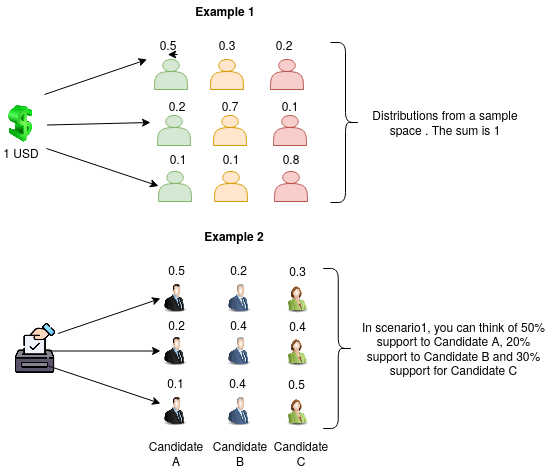
Example 2- Similarly, let’s say you want to predict how likely people are to vote for three candidates. As shown in above figure, in scenario 1, you believe A (50% votes) and C (30%) are more popular than B (20%).
Mathematical Explanation
The probability density function (PDF) for the Dirichlet distribution is defined as:

In above formula-
x1,x2,...,xK are the proportions (which must sum to 1).
α1,α2,…,αK are the parameters for each category.
Γ is the Gamma function .
Understanding alpha (α) parameters
The Dirichlet distribution is controlled by a set of numbers called parameters, written as α=[α1,α2,…,αK]. These parameters decide how balanced or extreme the distribution of probabilities will be.
Uniform Distribution
α =1: All combinations are equally likely.
When all αi=1, the PDF simplifies, making all combinations of probabilities equally likely. Lets understand this by code-
# Import libs
import numpy as np
import matplotlib.pyplot as plt
from scipy.stats import dirichlet
# Plot the samples on a 2D simplex (triangular plot)
# For more on triangular/simplex and barycentric plots-
# https://en.wikipedia.org/wiki/Ternary_plot
def plot_simplex(samples):
fig = plt.figure(figsize=(8, 6))
ax = fig.add_subplot(111)
# Convert to barycentric coordinates for plotting
x = samples[:, 0] + 0.5 * samples[:, 1]
y = np.sqrt(3) / 2 * samples[:, 1]
ax.scatter(x, y, alpha=0.1, edgecolor='k')
ax.set_title('Samples from Dirichlet Distribution')
plt.show()
# Parameters for Dirichlet distribution
alpha = [1, 1, 1]
# Generate samples
samples_uniform = dirichlet.rvs(alpha, size=5000)
plot_simplex(samples_uniform)
All combinations are equally likely. This is called a uniform distribution, meaning each possible probability scenario (like [0.3,.0.,0.4] or [0.5,0.2, 0.3] ) is equally likely. Think of it as having no prior bias toward any specific way of distributing probabilities. Basically you have no preference for how the votes are split. Any division is equally acceptable. Thats the plot shows a dense scatter across the entire simplex (triangle). There is no bias toward any specific outcome.
Balanced Distribution
When α >1: All combinations are equally likely.
Larger α values (all equal) favor more balanced distributions near the center of the simplex. For Example: Think of distributing votes among candidates where you expect relatively even support among them, though not perfectly strict
# Parameters for Dirichlet distribution
alpha = [6, 6, 6]

# Generate samples
samples_balanced = dirichlet.rvs(alpha, size=5000)

plot_simplex(samples_balanced)
Probabilities are more evenly distributed and cluster around the center of the triangle ([0.33,0.33,0.33]). The samples favor balanced scenarios where categories share probabilities evenly.
Skewed Distribution
Smaller values of α <1 favor extreme outcomes. One category tends to dominate, while others shrink toward zero. Example: In elections, perhaps one candidate might unexpectedly take the majority of votes.
# Parameters for Dirichlet distribution
alpha = [0.8, 0.3, 0.3]

# Generate samples
samples_skewed = dirichlet.rvs(alpha, size=5000)

plot_simplex(samples_skewed)
The distribution favors extreme points. You can see more samples near the vertices of the triangle, indicating that one category dominates while the others receive very little.
Why this is happening???
Dirichlet samples are derived by generating Gamma-distributed random variables and normalizing them.
Basically-
Larger α values produce Gamma samples with less variance and values clustered near the center.
Smaller α values result in more extreme values.
from scipy.stats import gamma
import numpy as np
import matplotlib.pyplot as plt

def plot_gamma_samples(alpha_value, size=5000):
    # Generate Gamma samples for three categories
    y1 = gamma.rvs(alpha_value, size=size)
    y2 = gamma.rvs(alpha_value, size=size)
    y3 = gamma.rvs(alpha_value, size=size)

    # Normalize them to sum to 1 (Dirichlet transformation )
    total = y1 + y2 + y3
    x1 = y1 / total
    x2 = y2 / total
    x3 = y3 / total

    # Plot the Gamma samples before normalization
    plt.figure(figsize=(8, 4))
    plt.hist(y1, bins=50, alpha=0.6, label=f'Gamma samples (alpha={alpha_value})')
    plt.legend()
    plt.title(f'Gamma Distribution for alpha={alpha_value}')
    plt.show()

    # Plot normalized Dirichlet samples
    plt.figure(figsize=(6, 3))
    plt.scatter(x1, x2, alpha=0.1, edgecolor='k')
    plt.title(f'Normalized Dirichlet Samples (alpha={alpha_value})')
    plt.show()

# Visualizing Gamma and Dirichlet samples for alpha values
plot_gamma_samples(1)  # Uniform
plot_gamma_samples(6)  # Balanced
plot_gamma_samples(0.5)  # Skewed
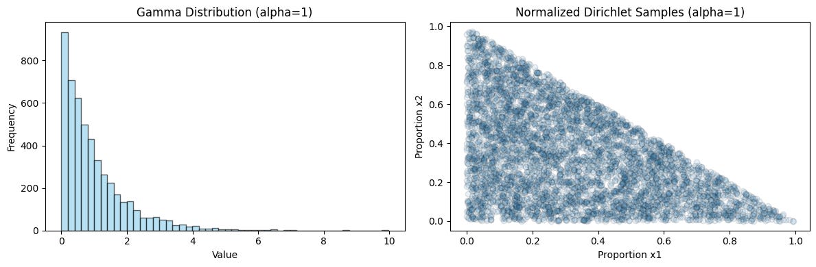


Gamma Distribution for α=1 (Uniform)
The Gamma samples are broadly distributed across different values.After normalization, the points scatter uniformly across the entire simplex.
Gamma Distribution for α=6 (Balanced)
The Gamma samples are tightly clustered, leading to balanced and less variable probabilities. After normalization, the points tend to cluster near the center.Gamma Distribution for α=0.5 (Skewed)
The Gamma samples are concentrated near small values, often close to zero. After normalization, the points scatter near the simplex vertices, indicating one dominant category.Gamma distribution defines the "weight" each category gets. By dividing by the total weight, itsd creates probability values for each category.
 α>1: Produces more balanced weights, favoring smoother, less extreme probabilities.
 α<1: Produces spiky, peaky weights, where some categories get much more weight than others.
In the next series, we will deep dive into different practical AI applications where Drichlet is used.